library(tidycensus)
library(tidyverse)
library(sf)
library(crsuggest)

census_api_key(Sys.getenv("CENSUS_API_KEY"), install = TRUE, overwrite = TRUE)A friend and I were recently discussing the proposed site for the DC Blox data center, which sits on the edge of my east side Indianapolis neighborhood (Irvington). We were curious about potential impacts on the nearby population and given my background in geospatial Census data analysis with R, I knew that I could generate some reasonable estimates.
After seeing how easy it was to do this type of analysis in R, but also that there were many ways to approach the problem, I wrote up the simplest workflow I could think of. The resulting code pulls Census block-level population data and clips it to a radius buffer around a single lat/long point.
The Approach
The core idea is simple:
- Pull 2020 Census block population data for Marion County using
tidycensus - Define a point (the proposed DC Blox site)
- Buffer that point to a given radius (0.5 mile and 1 mile)
- Find all Census blocks that intersect each buffer
- Sum the population
Census blocks are the smallest geographic unit the Census Bureau publishes population data for, which makes them ideal for this kind of proximity analysis. You won’t get perfect precision — a block that straddles the buffer boundary gets counted in full with my simple methodology — but for a back-of-the-envelope population impact estimate, blocks are far more accurate than using tracts or zip codes.
Note
It’s important to point out that the Census Bureau uses something called “differential privacy” to intentionally scramble geographic data with low counts to protect individual privacy. It is possible that some of the blocks in this analysis have inaccurate counts due to this practice, but addressing that issue is outside the scope of this blog post.
The Code
Setup and Data
First, load packages and authenticate with the Census API. I store my key in a .Renviron file so it never ends up in version-controlled code. For more on how to use the tidycensus package, read my blog post on that topic.
Now pull 2020 decennial population counts at the block level for Marion County, Indiana (Indianapolis). The geometry = TRUE argument returns the block polygons alongside the population data, giving us a spatial dataframe ready for analysis.
pop_blocks <- get_decennial(
  geography = "block",
  variables = "P1_001N",
  state = "IN",
  county = "Marion",
  year = 2020,
  sumfile = "pl",
  geometry = TRUE
)
It is important to adjust geospatial data to an appropriate projection, particularly when overlaying data from multiple sources as we will do later. The crsggest package is invaluable when it comes to this task.
# find best projection for our data
suggest_crs(pop_blocks, limit = 3)
Looks like 7328 is the best suggested option according to the package. We will use that throughout the analysis.
# Transform to a Marion County projected CRS for accurate distance calculations
pop_blocks <- pop_blocks %>% st_transform(7328)
Also pull in street centerlines for the map background — these help orient the viewer without needing a tile basemap. This part is not necessary, but I think it makes the map look better. I got streetlines from the City of Indianapolis website.
streets <- read_sf("Street_Centerlines/Street_Centerlines.shp") %>%
  st_transform(7328)
Define the Site and Buffers
The proposed DC Blox site is located just east of Irvington at approximately -86.052667 longitude, 39.767444 latitude. I estimated this by looking at the proposed site map and creating a point on Google Maps.
I created the point using the st_point function from the sf package and then created buffers at both 0.5 mile and 1 mile using the st_buffer function.
pt <- st_sfc(
  st_point(c(-86.052667, 39.767444)),
  crs = 4326
)

pt_proj <- st_transform(pt, 7328)

# CRS 7328 uses US survey feet
# 0.5 mile = 2,640 ft | 1 mile = 5,280 ft
buff_half <- st_buffer(pt_proj, dist = 2640)
buff_one  <- st_buffer(pt_proj, dist = 5280)

# Slightly wider street clip so the maps have breathing room
buff_streets <- st_buffer(pt_proj, dist = 8000)
buffer_streets <- streets[buff_streets, ]
Clip Blocks to Each Buffer
blocks_half <- pop_blocks[buff_half, ]
blocks_one  <- pop_blocks[buff_one, ]
The [buffer, ] syntax is sf’s spatial subsetting shorthand — it returns every row in pop_blocks whose geometry intersects the buffer polygon. This is the simplest way to approximate blocks that are “within” the radius.
Maps
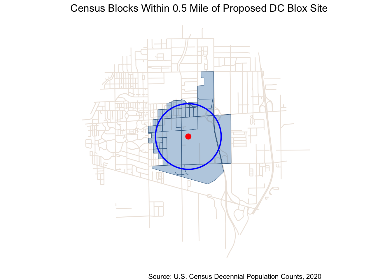
Half-Mile Radius
ggplot() +
  geom_sf(data = buffer_streets, fill = NA, color = "seashell2") +
  geom_sf(data = blocks_half, fill = "steelblue", alpha = 0.4, color = "steelblue4", linewidth = 0.2) +
  geom_sf(data = buff_half, fill = NA, color = "blue", linewidth = 0.8) +
  geom_sf(data = pt_proj, color = "red", size = 3) +
  theme_void() +
  labs(
    title = "Census Blocks Within 0.5 Mile of Proposed DC Blox Site",
    caption = "Source: U.S. Census Decennial Population Counts, 2020"
  )
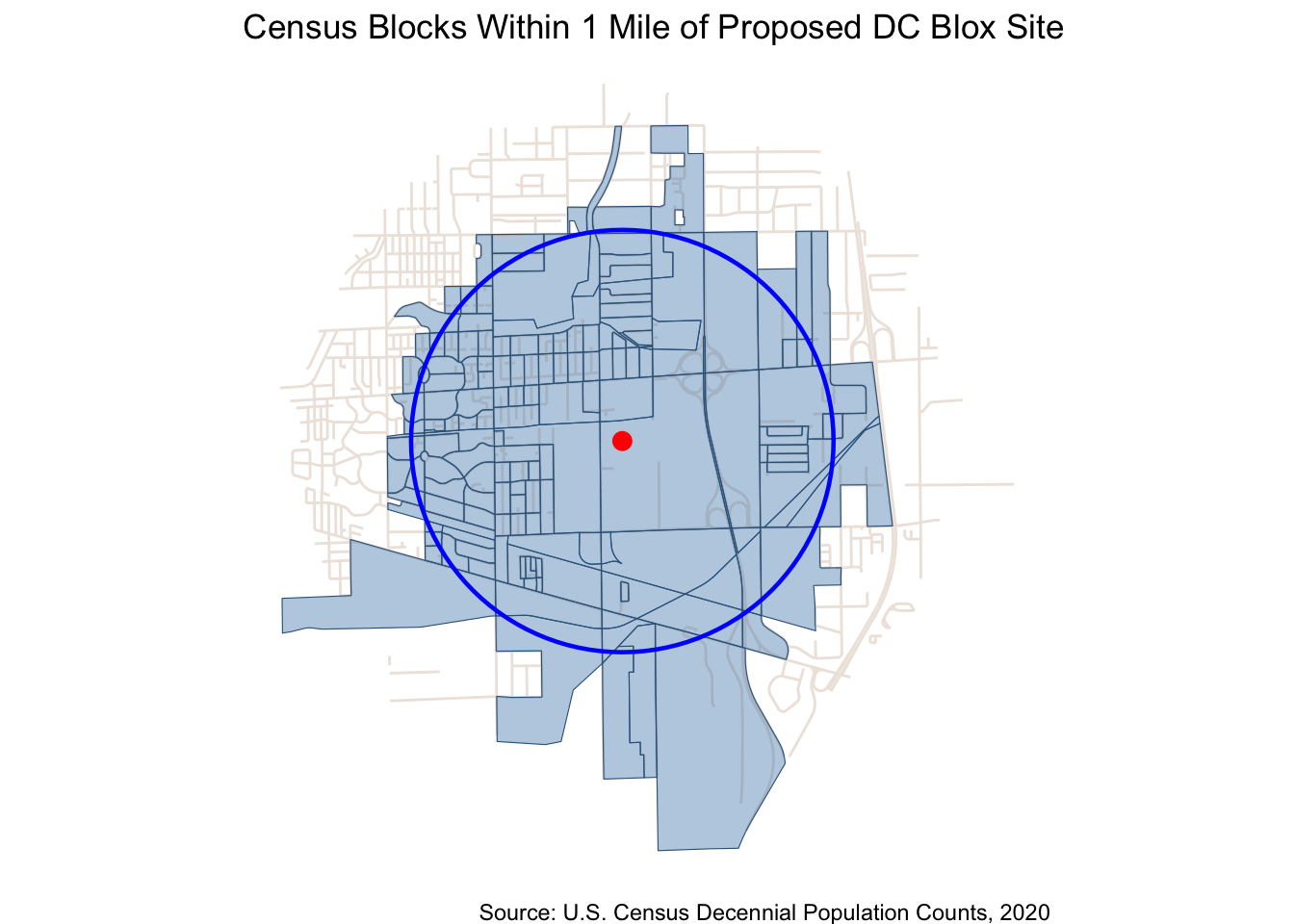
One-Mile Radius
ggplot() +
  geom_sf(data = buffer_streets, fill = NA, color = "seashell2") +
  geom_sf(data = blocks_one, fill = "steelblue", alpha = 0.4, color = "steelblue4", linewidth = 0.2) +
  geom_sf(data = buff_one, fill = NA, color = "blue", linewidth = 0.8) +
  geom_sf(data = pt_proj, color = "red", size = 3) +
  theme_void() +
  labs(
    title = "Census Blocks Within 1 Mile of Proposed DC Blox Site",
    caption = "Source: U.S. Census Decennial Population Counts, 2020"
  )
Population by Radius
radius_pop <- tibble(
  Radius = c("0.5 Mile", "1 Mile"),
  Population = c(
    sum(blocks_half$value),
    sum(blocks_one$value)
  )
)

ggplot(radius_pop, aes(x = Radius, y = Population, fill = Radius)) +
  geom_col() +
  geom_text(aes(label = scales::comma(Population)), vjust = -0.5) +
  scale_fill_manual(values = c("0.5 Mile" = "steelblue", "1 Mile" = "steelblue4")) +
  scale_y_continuous(labels = scales::comma, expand = expansion(mult = c(0, 0.1))) +
  labs(
    title = "Population Near Proposed DC Blox Site",
    subtitle = "By radius from site, Census blocks intersecting buffer",
    x = NULL,
    y = "Population",
    caption = "Source: U.S. Census Decennial Population Counts, 2020"
  ) +
  theme_minimal() +
  theme(legend.position = "none")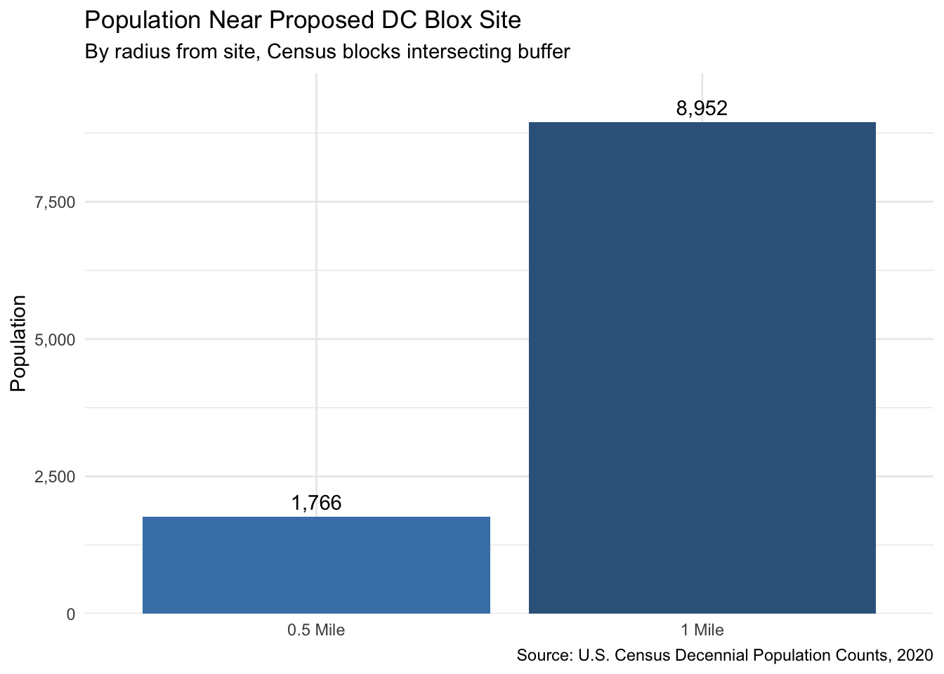
Potential Population Impact
Looking at the maps, its clear that the area just south and east of the proposed site have very few residential neighborhoods and a potentially small population impact. Just north and west of the site, however, are fairly dense (more blocks generally means more people). The result is nearly 2K people living within a half-mile radius of the site and 9K within 1 mile.
Wrapping Up
This analysis pattern–tidycensus + sf buffer + spatial subsetting–is straightforward and produces impact estimates quickly. It takes maybe 50 lines of R to go from a lat/long coordinate to a population estimate with geographic context. If you want to swap in a different location, you only need to change the point coordinates and re-run — the rest of the workflow is completely portable.